Power analysis before data collection — in base R

You don’t need special software to plan a sample size. power.t.test() and a power curve answer the question in ten lines of R.

The most expensive statistical mistake is made before any data exist: recruiting too few participants to detect the effect you care about. The fix costs ten lines of base R — no add-on packages, no point-and-click software.

The one-liner

Suppose we plan a two-group trial and consider a standardized difference of d = 0.5 (a “medium” effect) clinically meaningful. How many participants per group for 80% power at α = .05?

power.t.test(delta = 0.5, sd = 1, sig.level = 0.05, power = 0.80)

     Two-sample t test power calculation 

              n = 63.76576
          delta = 0.5
             sd = 1
      sig.level = 0.05
          power = 0.8
    alternative = two.sided

NOTE: n is number in *each* group

About 64 per group. The same function inverts in any direction — fix n and it returns the power, fix power and n and it returns the smallest detectable effect.

The more honest answer: a power curve

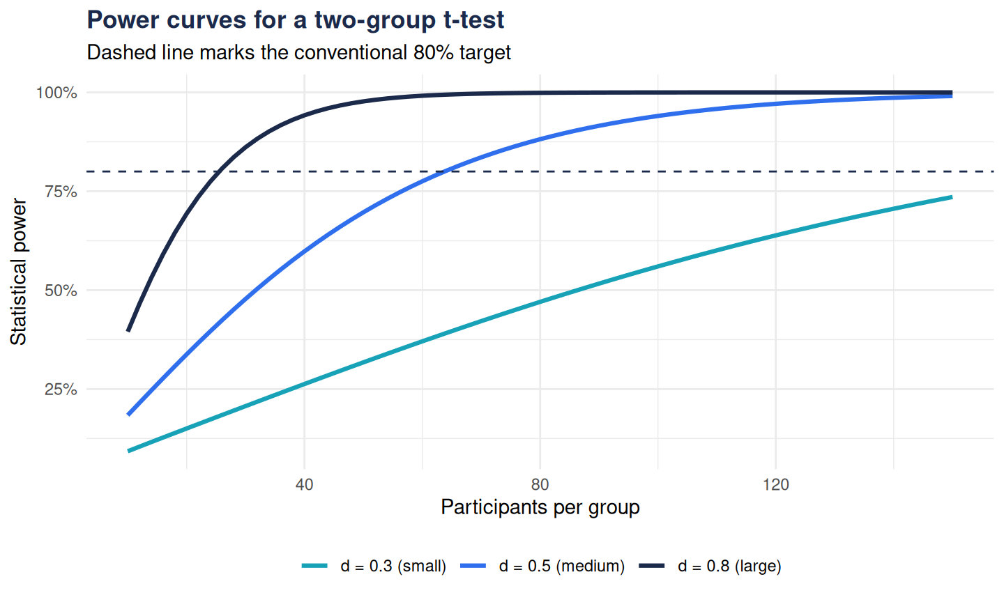
A single number hides how sensitive the design is to your effect-size guess. A curve makes the trade-off visible:

library(ggplot2)

grid <- expand.grid(
  n = seq(10, 150, by = 2),
  d = c(0.3, 0.5, 0.8)
)
grid$power <- mapply(
  function(n, d) power.t.test(n = n, delta = d)$power,
  grid$n, grid$d
)

ggplot(grid, aes(n, power, colour = factor(d))) +
  geom_line(linewidth = 1.1) +
  geom_hline(yintercept = 0.80, linetype = "dashed", colour = "#1b2a4a") +
  scale_colour_manual(
    values = c("#17a2b8", "#2f6fed", "#1b2a4a"),
    labels = c("d = 0.3 (small)", "d = 0.5 (medium)", "d = 0.8 (large)")
  ) +
  scale_y_continuous(labels = scales::percent) +
  labs(
    title = "Power curves for a two-group t-test",
    subtitle = "Dashed line marks the conventional 80% target",
    x = "Participants per group", y = "Statistical power", colour = NULL
  ) +
  theme_minimal() +
  theme(legend.position = "bottom",
        plot.title = element_text(face = "bold", colour = "#1b2a4a"))

Figure 1

The curve tells the real story: if the true effect is small (d = 0.3), even 150 per group leaves you underpowered — and if the budget only allows 30 per group, you are implicitly betting on a large effect.

Beyond the t-test

Base R also ships power.prop.test() for two proportions and power.anova.test() for one-way ANOVA. For more complex designs — mixed models, survival endpoints, cluster randomization — the honest tool is simulation: generate data under your assumed model a few thousand times and count how often the analysis detects the effect. That is a topic for a future post.

Planning a study and unsure about the numbers? We do this for a living.