One-way ANOVA in R with post-hoc tests

Run a one-way ANOVA in R, then use Tukey’s HSD to find which groups actually differ — with the multiple-comparison correction that keeps your error rate honest.

ANOVA tells you whether any group differs; a post-hoc test tells you which. Do the second step properly and you avoid inflating your false-positive rate. (For when to use ANOVA at all, see t-test vs ANOVA.)

Step 1: the ANOVA

We’ll use the built-in PlantGrowth data — plant yields under a control and two treatments:

fit <- aov(weight ~ group, data = PlantGrowth)
summary(fit)

            Df Sum Sq Mean Sq F value Pr(>F)  
group        2  3.766  1.8832   4.846 0.0159 *
Residuals   27 10.492  0.3886                 
---
Signif. codes:  0 '***' 0.001 '**' 0.01 '*' 0.05 '.' 0.1 ' ' 1

A small p-value for group says the groups are not all equal — but not which pair drives it.

Step 2: Tukey’s HSD

Never just run a bunch of t-tests here. Tukey’s Honest Significant Difference compares every pair while controlling the family-wise error rate:

TukeyHSD(fit)

  Tukey multiple comparisons of means
    95% family-wise confidence level

Fit: aov(formula = weight ~ group, data = PlantGrowth)

$group
            diff        lwr       upr     p adj
trt1-ctrl -0.371 -1.0622161 0.3202161 0.3908711
trt2-ctrl  0.494 -0.1972161 1.1852161 0.1979960
trt2-trt1  0.865  0.1737839 1.5562161 0.0120064

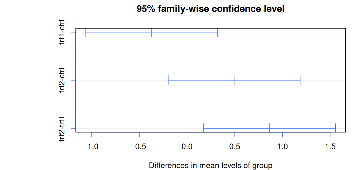
Each row is a pairwise difference with an adjusted confidence interval and p-value. Any interval that excludes zero is a significant difference.

par(mar = c(4, 8, 3, 1), family = "sans")
plot(TukeyHSD(fit), col = "#2f6fed")

Figure 1

Intervals crossing the dashed zero line are not significant; those entirely to one side are.

Before you trust it

ANOVA assumes roughly normal residuals and similar variances across groups. Check the residuals (plot(fit)) and normality; if variances differ badly, use oneway.test() (Welch) instead, and if normality fails, the Kruskal–Wallis test.

---

Running group comparisons in your data? We’ll handle the assumptions and the write-up.